YeoJohnsonTransformer#

The Yeo-Johnson transformation is an extension of the Box-Cox transformation, enabling power transformations on variables with zero and negative values, in addition to positive values.

The Box-Cox transformation, on the other hand, is suitable for numeric variables that are strictly positive. When variables include negative values, we have two options:

  • shift the distribution toward positive values by adding a constant

  • use the Yeo-Johnson transformation

The Yeo-Johnson transformation is defined as:


../../_images/yeojohnsonformula.png

where Y is the independent variable and λ is the transformation parameter.

Uses of the Yeo-Johnson and Box-Cox transformation#

Both the Yeo-Johnson and Box-Cox transformations automate the process of identifying the optimal power transformation to approximate a Gaussian distribution. They evaluate various power transformations, including the logarithmic and reciprocal functions, estimating the transformation parameter through maximum likelihood.

These transformations are commonly applied during data preprocessing, particularly when parametric statistical tests or linear models for regression are employed. Such tests and models often have underlying assumptions about the data that may not be inherently satisfied, making these transformations essential for meeting those assumptions.

Yeo-Johnson vs Box-Cox transformation#

How does the Yeo-Johnson transformation relate to the Box-Cox transformation?

The Yeo-Johnson transformation extends the Box-Cox transformation to handle variables with zero, negative, and positive values.

  • For strictly positive values: The Yeo-Johnson transformation is equivalent to the Box-Cox transformation applied to (X + 1).

  • For strictly negative values: The Yeo-Johnson transformation corresponds to the Box-Cox transformation applied to (-X + 1) with a power of (2 — λ), where λ is the transformation parameter.

  • For variables with both positive and negative values: The Yeo-Johnson transformation combines the two approaches, using different powers for the positive and negative segments of the variable.

To apply the Yeo-Johnson transformation in Python, you can use scipy.stats.yeojohnson, which can transform one variable at a time. For transforming multiple variables simultaneously, libraries like scikit-klearn and Feature-engine are more suitable.

The YeoJohnsonTransformer#

Feature-engine’s YeoJohnsonTransformer() applies the Yeo-Johnson transformation to numeric variables.

Under the hood, YeoJohnsonTransformer() uses scipy.stats.yeojohnson to apply the transformations to each variable.

Python Implementation#

In this section, we will apply the Yeo-Johnson transformation to several variables from the Ames house prices dataset. After performing the transformations, we will carry out data analysis to understand the impact on the variable distributions.

Let’s begin by importing the necessary libraries and transformers, loading the dataset, and splitting it into training and testing sets.

import numpy as np
import pandas as pd
import matplotlib.pyplot as plt
from sklearn.datasets import fetch_openml
from sklearn.model_selection import train_test_split
from feature_engine.transformation import YeoJohnsonTransformer

# Load dataset
data = fetch_openml(name='house_prices', as_frame=True)
data = data.frame

# Separate into train and test sets
X_train, X_test, y_train, y_test =  train_test_split(
            data.drop(['Id', 'SalePrice'], axis=1),
            data['SalePrice'], test_size=0.3, random_state=0)

X_train.head()

In the following output we see the predictor variables of the house prices dataset:

      MSSubClass MSZoning  LotFrontage  LotArea Street Alley LotShape  \
254           20       RL         70.0     8400   Pave   NaN      Reg
1066          60       RL         59.0     7837   Pave   NaN      IR1
638           30       RL         67.0     8777   Pave   NaN      Reg
799           50       RL         60.0     7200   Pave   NaN      Reg
380           50       RL         50.0     5000   Pave  Pave      Reg

     LandContour Utilities LotConfig  ... ScreenPorch PoolArea PoolQC  Fence  \
254          Lvl    AllPub    Inside  ...           0        0    NaN    NaN
1066         Lvl    AllPub    Inside  ...           0        0    NaN    NaN
638          Lvl    AllPub    Inside  ...           0        0    NaN  MnPrv
799          Lvl    AllPub    Corner  ...           0        0    NaN  MnPrv
380          Lvl    AllPub    Inside  ...           0        0    NaN    NaN

     MiscFeature MiscVal  MoSold  YrSold  SaleType  SaleCondition
254          NaN       0       6    2010        WD         Normal
1066         NaN       0       5    2009        WD         Normal
638          NaN       0       5    2008        WD         Normal
799          NaN       0       6    2007        WD         Normal
380          NaN       0       5    2010        WD         Normal

[5 rows x 79 columns]

Let’s now set up the transformer to apply the Yeo-Johnson transformation to 2 variables; LotArea and GrLivArea:

tf = YeoJohnsonTransformer(variables = ['LotArea', 'GrLivArea'])

tf.fit(X_train)

With fit(), YeoJohnsonTransformer() learns the optimal lambda for the yeo-johnson power transformation. We can inspect these values as follows:

tf.lambda_dict_

We see the optimal lambda values below:

{'LotArea': 0.02258978732751055, 'GrLivArea': 0.06781061353154169}

We can now go ahead and apply the data transformation to get closer to normal distributions.

train_t = tf.transform(X_train)
test_t = tf.transform(X_test)

We’ll check out the effect of the transformation in the next section.

Effect of the transformation on the variable distribution#

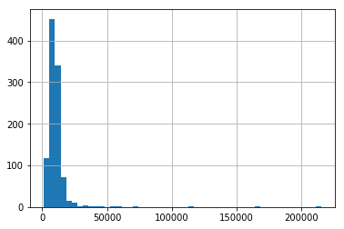
Let’s carry out an analysis of transformations. We’ll explore the variables distribution before and after applying the transformation described by Yeo and Johnson.

Let’s make histograms of the original data to check out the original variables distribution:

X_train[['LotArea', 'GrLivArea']].hist(bins=50, figsize=(10,4))
plt.show()

In the following image, we can observe the skewness in the distribution of ‘LotArea’ and ‘GrLivArea’ in the original data:

../../_images/untransformedcoupleYJ.png


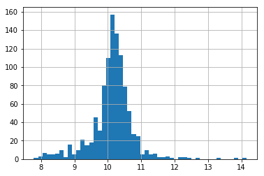
Now, let’s plot histograms of the transformed variables:

train_t[['LotArea', 'GrLivArea']].hist(bins=50, figsize=(10,4))
plt.show()

We see that in the transformed data, both variables have a more symmetric, Gaussian-like distribution.

../../_images/transformedcoupleYJ.png


Recovering the original data#

After applying the Yeo-Johnson transformation, we can restore the original data representation, that is, the original variable values, using the inverse_transform method.

train_unt = tf.inverse_transform(train_t)
test_unt = tf.inverse_transform(test_t)

Additional resources#

You can find more details about the YeoJohnsonTransformer() here:

For more details about this and other feature engineering methods check out these resources:

../../_images/feml.png

Feature Engineering for Machine Learning#


Or read our book:

../../_images/cookbook.png

Python Feature Engineering Cookbook#


Both our book and course are suitable for beginners and more advanced data scientists alike. By purchasing them you are supporting Sole, the main developer of Feature-engine.