EndTailImputer

The EndTailImputer() replaces missing data with a value at the end of the distribution. The value can be determined using the mean plus or minus a number of times the standard deviation, or using the inter-quartile range proximity rule. The value can also be determined as a factor of the maximum value.

You decide whether the missing data should be placed at the right or left tail of the variable distribution.

Tip

The EndTailImputer() “automates” the work of the ArbitraryNumberImputer() by automatically finding “arbitrary values” far out at the end of the variable distributions.

EndTailImputer() works only with numerical variables. You can impute only a subset of the variables in the data by passing the variable names in a list. Alternatively, the imputer will automatically select all numerical variables in the train set.

Python implementation

Below a code example using the house prices dataset.

First, let’s load the data and separate it into train and test:

import matplotlib.pyplot as plt
from sklearn.datasets import fetch_openml
from sklearn.model_selection import train_test_split

from feature_engine.imputation import EndTailImputer

# Load dataset
X, y = fetch_openml(
    name='house_prices',
    version=1,
    return_X_y=True,
    as_frame=True,
    parser='auto',
)

# Separate into train and test sets
X_train, X_test, y_train, y_test = train_test_split(
    X,
    y,
    test_size=0.3,
    random_state=0,
)

Now we set up the EndTailImputer() to impute only 2 variables from the dataset. We instruct the imputer to find the imputation values using the mean plus 3 times the standard deviation as follows:

# set up the imputer
tail_imputer = EndTailImputer(
    imputation_method='gaussian',
    tail='right',
    fold=3,
    variables=['LotFrontage', 'MasVnrArea']
)

# fit the imputer
tail_imputer.fit(X_train)

With fit, the EndTailImputer() learned the imputation values for the indicated variables and stored it in one of its attributes. We can now go ahead and impute both the train and the test sets.

# transform the data
train_t = tail_imputer.transform(X_train)
test_t = tail_imputer.transform(X_test)

Note that after the imputation, if the percentage of missing values is relatively large, the variable distribution will differ from the original one.

Let’s create a density plot to observe the change in the distribution:

fig = plt.figure()
ax = fig.add_subplot(111)
X_train['LotFrontage'].plot(kind='kde', ax=ax)
train_t['LotFrontage'].plot(kind='kde', ax=ax, color='red')
lines, labels = ax.get_legend_handles_labels()
ax.legend(lines, labels, loc='best')

In the following image, we see the distribution of LotFrontage before and after the imputation (in red the imputed variable):

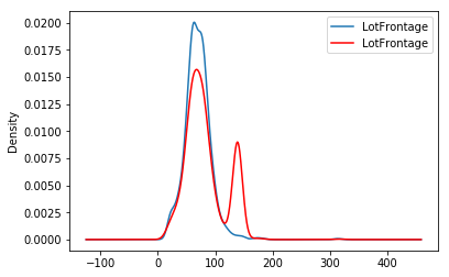
The second peak corresponds to the missing data, which were replaced with a value at that side of the distribution.

Additional resources

For tutorials about missing data imputation methods check out these resources:

• Feature Engineering for Machine Learning, online course.

• Feature Engineering for Time Series Forecasting, online course.

• Python Feature Engineering Cookbook, book.

Both our book and courses are suitable for beginners and more advanced data scientists alike. By purchasing them you are supporting Sole, the main developer of Feature-engine.