ProbeFeatureSelection#

ProbeFeatureSelection() adds one or more random variables to the dataframe. Next it derives the feature importance for each variable, including the probe features. Finally, it removes those features whose importance is lower than the probes.

Deriving feature importance#

ProbeFeatureSelection() has 2 strategies to derive feature importance.

In the collective strategy, ProbeFeatureSelection() trains one machine learning model using all the variables plus the probe features, and then derives the feature importance from the fitted model. This feature importance is given by the coefficients of linear models or the feature importance derived from tree-based algorithms.

In the individual feature strategy, ProbeFeatureSelection() trains one machine learning model per feature and per probe, and then, the feature importance is given by the performance of that single feature model. Here, the importance is given by any performance metric chosen by you.

Both strategies have advantages and limitations. If the features are correlated, the feature importance value returned by the coefficients of a linear model, or derived from a decision tree, will appear to be smaller than if the feature was used to train a model individually. Hence, potentially important features might be lost to the probes due to these seemingly low importance values resulting from correlation.

On the other hand, training models using individual features, does not allow to detect feature interactions and does not remove redundant variables.

In addition, keep in mind that the importance derived tree-based models is biased towards features with high cardinality. Hence, continuous features will seem to be more important than discrete variables. If your features are discrete and your probes continuous, you could be removing important features accidentally.

Selecting features#

After assigning a value of feature importance to each feature, including the probes, ProbeFeatureSelection() will select those variables whose importance is greater than the mean importance of all probes.

Feature selection process#

This is how ProbeFeatureSelection() selects features using the collective strategy:

Add 1 or more random features to the dataset
Train a machine learning model using all features including the random ones
Derive feature importance from the fitted model
Take the average importance of the random features
Select features whose importance is greater than the importance of the random variables (step 4)

This is how ProbeFeatureSelection() selects features using the individual feature strategy:

Add 1 or more random features to the dataset
Train a machine learning per feature and per probe
Determine the feature importance as the performance of the single feature model
Take the average importance of the random features
Select features whose importance is greater than the importance of the random variables (step 4)

Rationale of probe feature selection#

One of the primary goals of feature selection is to remove noise from the dataset. A randomly generated variable, i.e., probe feature, inherently possesses a high level of noise. Consequently, any variable with less importance than a probe feature is assumed to be noise and can be discarded from the dataset.

Distribution of the probe features#

When initiating the ProbeFeatureSelection() class, you have the option to select which distribution is to be assumed to create the probe feature(s), as well as the number of probe features to create.

The possible distributions are ‘normal’, ‘binary’, ‘uniform’, or ‘all’. ‘all’ creates 1 or more probe features comprised of each distribution type, i.e., normal, binomial, and uniform. So, if you selected ‘all’ and are creating 9 probe features, you will have 3 probes for each distribution.

The distribution matters. Tree-based models tend to give more importance to highly cardinal features. Hence, probes created from a uniform or normal distribution will display a greater importance than probes extracted from a binomial distribution when using these models.

Python examples#

Let’s see how to use this transformer to select variables from UC Irvine’s Breast Cancer Wisconsin (Diagnostic) dataset, which can be found here. We will use Scikit-learn to load the dataset. This dataset concerns breast cancer diagnoses. The target variable is binary, i.e., malignant or benign. The data is solely comprised of numerical data.

Let’s import the required libraries and classes:

import pandas as pd
from sklearn.datasets import load_breast_cancer
from sklearn.ensemble import RandomForestClassifier
from sklearn.model_selection import train_test_split
from feature_engine.selection import ProbeFeatureSelection

Let’s now load the cancer diagnostic data:

cancer_X, cancer_y = load_breast_cancer(return_X_y=True, as_frame=True)

Let’s check the shape of cancer_X:

print(cancer_X.shape)

We see that the dataset is comprised of 569 observations and 30 features:

(569, 30)

Let’s now split the data into train and test sets:

# separate train and test sets
X_train, X_test, y_train, y_test = train_test_split(
    cancer_X,
    cancer_y,
    test_size=0.2,
    random_state=3
)

X_train.shape, X_test.shape

We see the size of the datasets below. Note that there are 30 features in both the training and test sets.

((455, 30), (114, 30))

Now, we set up ProbeFeatureSelection() to select features using the collective strategy.

We will pass RandomForestClassifier() as the estimator. We will use precision as the scoring parameter and 5 as cv parameter, both parameters to be used in the cross validation.

In this example, we will introduce just 1 random feature with a normal distribution. Thus, we pass 1 for the n_probes parameter and normal as the distribution.

sel = ProbeFeatureSelection(
    estimator=RandomForestClassifier(),
    variables=None,
    scoring="precision",
    n_probes=1,
    distribution="normal",
    cv=5,
    random_state=150,
    confirm_variables=False
)

sel.fit(X_train, y_train)

With fit(), the transformer:

creates n_probes number of probe features using provided distribution(s)
uses cross-validation to fit the provided estimator
calculates the feature importance score for each variable, including probe features
if there are multiple probe features, the transformer calculates the average importance score
identifies features to drop because their importance scores are less than that of the probe feature(s)

Analysing the probes#

In the attribute probe_features, we find the pseudo-randomly generated variable(s):

sel.probe_features_.head()

       gaussian_probe_0
       -0.694150
        1.171840
        1.074892
        1.698733
        0.498702

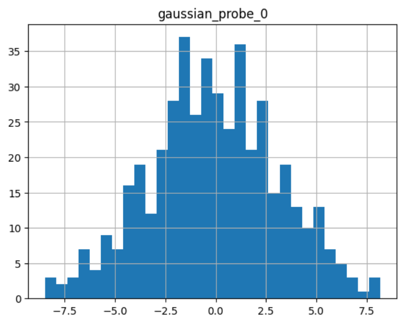
We can go ahead and display a histogram of the probe feature:

sel.probe_features_.hist(bins=30)

As we can see, it shows a normal distribution:

Analysing the feature importance#

The attribute feature_importances_ shows each variable’s feature importance:

sel.feature_importances_.head()

These are the importance for the first 5 features:

mean radius        0.058463
mean texture       0.011953
mean perimeter     0.069516
mean area          0.050947
mean smoothness    0.004974
dtype: float64

At the end of the series, we see the importance of the probe feature:

sel.feature_importances_.tail()

These are the importance of the last 5 features including the probe:

worst concavity            0.037844
worst concave points       0.102769
worst symmetry             0.011587
worst fractal dimension    0.007456
gaussian_probe_0           0.003783
dtype: float64

In the attribute feature_importances_std_ we find the standard deviation of the feature importance, which we can use for data analysis:

sel.feature_importances_std_.head()

These are the standard deviations for the first 5 features:

mean radius        0.013648
mean texture       0.002571
mean perimeter     0.025189
mean area          0.010173
mean smoothness    0.001650
dtype: float64

We can go ahead and plot bar plots with the feature importance and the standard deviation:

r = pd.concat([
    sel.feature_importances_,
    sel.feature_importances_std_
], axis=1)

r.columns = ["mean", "std"]

r.sort_values("mean", ascending=False)["mean"].plot.bar(
    yerr=[r['std'], r['std']], subplots=True, figsize=(15,6)
)
plt.title("Feature importance derived from the random forests")
plt.ylabel("Feature importance")
plt.show()

In the following image, we see the importance of each feature, including the probe:

Selected features#

In the attribute features_to_drop_, we find the variables that were not selected:

sel.features_to_drop_

These are the variables that will be removed from the dataframe:

['mean symmetry',
 'mean fractal dimension',
 'texture error',
 'smoothness error',
 'concave points error',
 'fractal dimension error']

We see that the features_to_drop_ have feature importance scores that are less than the probe feature’s score:

sel.feature_importances_.loc[sel.features_to_drop_+["gaussian_probe_0"]]

The previous command returns the following output:

mean symmetry              0.003698
mean fractal dimension     0.003455
texture error              0.003595
smoothness error           0.003333
concave points error       0.003548
fractal dimension error    0.003576
gaussian_probe_0           0.003783

Dropping features from the data#

With transform(), we can go ahead and drop the six features with feature importance score smaller than gaussian_probe_0 variable:

Xtr = sel.transform(X_test)

Xtr.shape

The final shape of the data after removing the features:

(114, 24)

Getting the name of the resulting features#

And, finally, we can also obtain the names of the features in the final transformed dataset:

sel.get_feature_names_out()

In the following output we see the name of the features that will be present in the transformed datasets:

['mean radius',
 'mean texture',
 'mean perimeter',
 'mean area',
 'mean smoothness',
 'mean compactness',
 'mean concavity',
 'mean concave points',
 'radius error',
 'perimeter error',
 'area error',
 'compactness error',
 'concavity error',
 'symmetry error',
 'worst radius',
 'worst texture',
 'worst perimeter',
 'worst area',
 'worst smoothness',
 'worst compactness',
 'worst concavity',
 'worst concave points',
 'worst symmetry',
 'worst fractal dimension']

For compatibility with Scikit-learn selection transformers, ProbeFeatureSelection() also supports the method get_support():

sel.get_support()

which returns the following output:

[True, True, True, True, True, True, True, True, False, False, True, False, True,
 True, False, True, True, False, True, False, True, True, True, True, True, True,
 True, True, True, True]

Using several probe features#

Let’s now repeat the selection process, but using more than 1 probe feature.

sel = ProbeFeatureSelection(
    estimator=RandomForestClassifier(),
    variables=None,
    scoring="precision",
    n_probes=3,
    distribution="all",
    cv=5,
    random_state=150,
    confirm_variables=False
)

sel.fit(X_train, y_train)

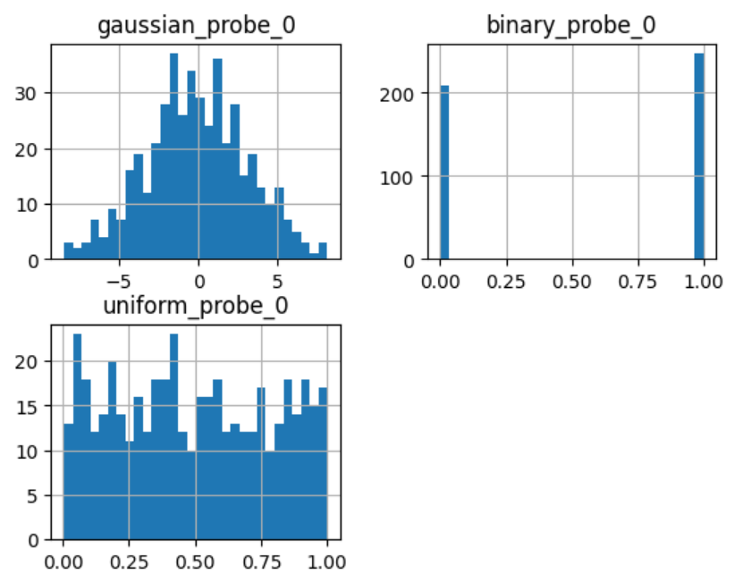
Let’s display the random features that the transformer created:

sel.probe_features_.head()

Here we find some example values of the probe features:

   gaussian_probe_0  binary_probe_0  uniform_probe_0
       -0.694150               1         0.983610
        1.171840               1         0.765628
        1.074892               1         0.991439
        1.698733               0         0.668574
        0.498702               0         0.192840

Let’s go ahead and plot histograms:

sel.probe_features_.hist(bins=30)
plt.show()

In the histograms we recognise the 3 well defined distributions:

Let’s display the importance of the random features

sel.feature_importances_.tail()

worst symmetry             0.009176
worst fractal dimension    0.007825
gaussian_probe_0           0.003765
binary_probe_0             0.000354
uniform_probe_0            0.002377
dtype: float64

We see that the binary feature has an extremely low importance, hence, when we take the average, the value is so small, that no feature will be dropped (remember random forests favouring highly cardinal features?):

sel.features_to_drop_

The previous command returns and empty list:

[]

It is important to select a suitable probe feature distribution when trying to remove variables. If most variables are continuous, introduce features with normal and uniform distributions. If you have one hot encoded features or sparse matrices, binary features might be a better option.

Using the individual feature strategy#

We will now repeat the process, but we will train a random forest per feature instead, and use the roc-auc as a measure of feature importance:

sel = ProbeFeatureSelection(
    estimator=RandomForestClassifier(n_estimators=5, random_state=1),
    variables=None,
    collective=False,
    scoring="roc_auc",
    n_probes=3,
    distribution="all",
    cv=5,
    random_state=150,
    confirm_variables=False
)

sel.fit(X_train, y_train)

We can now go ahead and plot the feature importance, including that of the probes:

r = pd.concat([
    sel.feature_importances_,
    sel.feature_importances_std_
], axis=1)

r.columns = ["mean", "std"]

r.sort_values("mean", ascending=False)["mean"].plot.bar(
    yerr=[r['std'], r['std']], subplots=True, figsize=(15,6)
)
plt.title("Feature importance derived from single feature models")
plt.ylabel("Feature importance - roc-auc")
plt.show()

In the following image we see the feature importance, including the probes:

../../_images/single_feature_probes_imp.png

When assessed individually, each feature seems to have a greater importance. Note that many of the features return roc-auc that are not significantly different from the probes (error bars overlaps). So, even if the transformer would not drop those features, we could decide to discard them after analysis of this plot.

Additional resources#

More info about this method can be found in these resources:

Kaggle Tips for Feature Engineering and Selection, by Gilberto Titericz.
Feature Selection: Beyond feature importance?, KDDNuggets.

For more details about this and other feature selection methods check out these resources:

Feature Selection for Machine Learning#

Or read our book:

Feature Selection in Machine Learning#

Both our book and course are suitable for beginners and more advanced data scientists alike. By purchasing them you are supporting Sole, the main developer of Feature-engine.

This site uses cookies