RandomSampleImputer

The RandomSampleImputer() replaces missing data with a random sample extracted from the variable. It works with both numerical and categorical variables. A list of variables can be indicated, or the imputer will automatically impute all variables in the dataset.

Note

The random samples used to replace missing values may vary from execution to execution. This may affect the results of your work. Thus, it is advisable to set a seed.

Setting the seed

There are 2 ways in which the seed can be set in RandomSampleImputer():

If seed = 'general' then the random_state can be either None or an integer. The random_state then provides the seed to use in the imputation. All observations will be imputed in one go with a single seed. This is equivalent to pandas.sample(n, random_state=seed) where n is the number of observations with missing data and seed is the number you entered in the random_state.

If seed = 'observation', then the random_state should be a variable name or a list of variable names. The seed will be calculated observation per observation, either by adding or multiplying the values of the variables indicated in the random_state. Then, a value will be extracted from the train set using that seed and used to replace the NAN in that particular observation. This is the equivalent of pandas.sample(1, random_state=var1+var2) if the seeding_method is set to add or pandas.sample(1, random_state=var1*var2) if the seeding_method is set to multiply.

For example, if the observation shows variables color: np.nan, height: 152, weight:52, and we set the imputer as:

RandomSampleImputer(
    random_state=['height', 'weight'],
    seed='observation',
    seeding_method='add',
)

the np.nan in the variable colour will be replaced using pandas sample as follows:

observation.sample(1, random_state=int(152+52))

Note

Note, if the variables indicated in the random_state list are not numerical the imputer will return an error. In addition, the variables indicated as seed should not contain missing values themselves.

Important for GDPR

This estimator stores a copy of the training set when the fit() method is called. Therefore, the object can become quite heavy. Also, it may not be GDPR compliant if your training data set contains Personal Information. Please check if this behaviour is allowed within your organisation.

Python implementation

Below a code example using the house prices dataset.

First, let’s load the data and separate it into train and test:

import matplotlib.pyplot as plt
from sklearn.datasets import fetch_openml
from sklearn.model_selection import train_test_split

from feature_engine.imputation import RandomSampleImputer

# Load dataset
data = fetch_openml(name='house_prices', as_frame=True)
data = data.frame

# Separate into train and test sets
X_train, X_test, y_train, y_test = train_test_split(
        data.drop(['Id', 'SalePrice'], axis=1),
        data['SalePrice'],
        test_size=0.3,
        random_state=0
)

In this example, we sample values at random, observation per observation, using as seed the value of the variable ‘MSSubClass’ plus the value of the variable ‘YrSold’. Note that the seed’s value is different for each observation.

The RandomSampleImputer() will impute all variables in the data, as we left the default value of the parameter variables to None.

# set up the imputer
imputer = RandomSampleImputer(
        random_state=['MSSubClass', 'YrSold'],
        seed='observation',
        seeding_method='add'
    )

# fit the imputer
imputer.fit(X_train)

With fit() the imputer stored a copy of X_train. And with transform, it will extract values at random from X_train to replace NA in the datasets indicated in the transform() method.

# transform the data
train_t = imputer.transform(X_train)
test_t = imputer.transform(X_test)

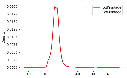
The beauty of the random sampler is that it preserves the original variable distribution.

Let’s check that out by creating a density plot:

fig = plt.figure()
ax = fig.add_subplot(111)
X_train['LotFrontage'].plot(kind='kde', ax=ax)
train_t['LotFrontage'].plot(kind='kde', ax=ax, color='red')
lines, labels = ax.get_legend_handles_labels()
ax.legend(lines, labels, loc='best')

In the following image we see the distribution of LotFrontage before and after the imputation (in red the imputed variable):

Additional resources

For tutorials about missing data imputation methods check out these resources:

• Feature Engineering for Machine Learning, online course.

• Feature Engineering for Time Series Forecasting, online course.

• Python Feature Engineering Cookbook, book.

Both our book and courses are suitable for beginners and more advanced data scientists alike. By purchasing them you are supporting Sole, the main developer of Feature-engine.