EqualWidthDiscretiser#
Equal width discretization consist of dividing continuous variables into intervals of equal width, calculated using the following formula:
Here, bins
is the number of intervals specified by the user and max(X)
and min(X)
are the minimum and maximum values
of the variable to discretize.
Discretization is a common data preprocessing technique used in data science. It’s also known as data binning (or simply “binning”).
Advantages and Limitations#
Equal binning discretization has some advantages and also shortcomings.
Advantages#
Some advantages of equal width binning:
Algorithm Efficiency: Enhances the performance of data mining and machine learning algorithms by providing a simplified representation of the dataset.
Outlier Management: Efficiently mitigates the effect of outliers by grouping them into the extreme bins, thus preserving the integrity of the main data distribution.
Data Smoothing: Helps smooth the data, reduces noise, and improves the model’s ability to generalize.
Limitations#
On the other hand, equal width discretzation can lead to a loss of information by aggregating data into broader categories. This is particularly concerning if the data in the same bin has predictive information about the target.
Let’s consider a binary classifier task using a decision tree model. A bin with a high proportion of both target categories would potentially impact the model’s performance in this scenario.
EqualWidthDiscretiser#
Feture-engine’s EqualWidthDiscretiser()
applies equal width discretization to numerical variables. It uses
the pandas.cut()
function under the hood to find the interval limits and then sort the continuous variables into
the bins.
You can specify the variables to be discretized by passing their names in a list when you set up the transformer. Alternatively,
EqualWidthDiscretiser()
will automatically infer the data types to compute the interval limits for all numeric
variables.
Optimal number of intervals: With EqualWidthDiscretiser()
, the user defines the number of bins. Smaller intervals
may be required if the variable is highly skewed or not continuous.
Integration with scikit-learn: EqualWidthDiscretiser()
and all other Feature-engine transformers seamlessly
integrate with scikit-learn pipelines.
Python code example#
In this section, we’ll show the main functionality of EqualWidthDiscretiser()
.
Load dataset#
In this example, we’ll use the Ames House Prices’ Dataset. First, let’s load the dataset and split it into train and test sets:
import matplotlib.pyplot as plt
from sklearn.datasets import fetch_openml
from sklearn.model_selection import train_test_split
from feature_engine.discretisation import EqualFrequencyDiscretiser
# Load dataset
X, y = fetch_openml(name='house_prices', version=1, return_X_y=True, as_frame=True)
X.set_index('Id', inplace=True)
# Separate into train and test sets
X_train, X_test, y_train, y_test = train_test_split(X, y, test_size=0.3, random_state=42)
Equal-width Discretization#
In this example, let’s discretize two variables, LotArea and GrLivArea, into 10 intervals of equal width:
# List the target numeric variables for equal-width discretization
TARGET_NUMERIC_FEATURES= ['LotArea','GrLivArea']
# Set up the discretization transformer
disc = EqualWidthDiscretiser(bins=10, variables=TARGET_NUMERIC_FEATURES)
# Fit the transformer
disc.fit(X_train)
Note that if we do not specify the variables (default=`None`), EqualWidthDiscretiser
will automatically infer
the data types to compute the interval limits for all numeric variables.
With the fit()
method, the discretizer learns the bin boundaries and saves them into a dictionary so we can use them
to transform unseen data:
# Learned limits for each variable
disc.binner_dict_
{'LotArea': [-inf,
22694.5,
44089.0,
65483.5,
86878.0,
108272.5,
129667.0,
151061.5,
172456.0,
193850.5,
inf],
'GrLivArea': [-inf,
864.8,
1395.6,
1926.3999999999999,
2457.2,
2988.0,
3518.7999999999997,
4049.5999999999995,
4580.4,
5111.2,
inf]}
Note that the lower and upper boundaries are set to -inf and inf, respectively. This behavior ensures that the transformer will be able to allocate to the extreme bins values that are smaller or greater than the observed minimum and maximum values in the training set.
EqualWidthDiscretiser
will not work in the presence of missing values. Therefore, we should either remove or
impute missing values before fitting the transformer.
# Transform the data (data discretization)
train_t = disc.transform(X_train)
test_t = disc.transform(X_test)
Let’s visualize the first rows of the raw data and the transformed data:
# Raw data
print(X_train[TARGET_NUMERIC_FEATURES].head())
Here we see the original variables:
LotArea GrLivArea
Id
136 10400 1682
1453 3675 1072
763 8640 1547
933 11670 1905
436 10667 1661
# Transformed data
print(train_t[TARGET_NUMERIC_FEATURES].head())
Here we observe the variables after discretization:
LotArea GrLivArea
Id
136 0 2
1453 0 1
763 0 2
933 0 2
436 0 2
The transformed data now contains discrete values corresponding to the ordered computed buckets (0 being the first and bins-1 the last).
Now, let’s check out the number of observations per bin by creating a bar plot:
train_t['GrLivArea'].value_counts().sort_index().plot.bar()
plt.ylabel('Number of houses')
plt.show()
As we see in the following image, the intervals contain different number of observations. It’s a similar output to a histogram:
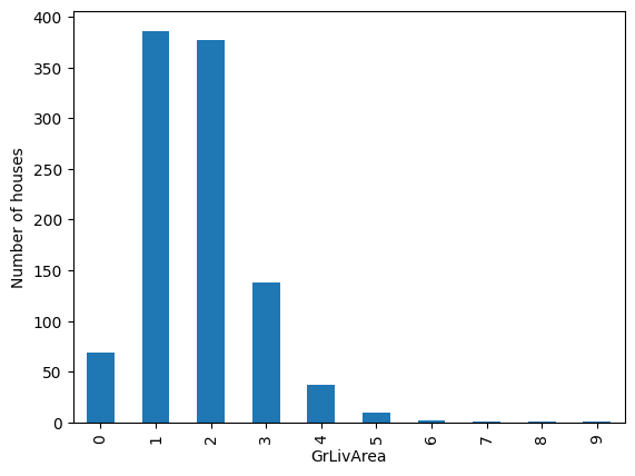
Equal width discretization does not improve the spread of values over the value range. If the variable is skewed, it will still be skewed after the discretization.
Finally, since the default value for the return_object
parameter is False
, the transformer outputs integer variables:
train_t[TARGET_NUMERIC_FEATURES].dtypes
LotArea int64
GrLivArea int64
dtype: object
Return variables as object#
Categorical encoders in Feature-engine are designed to work by default with variables of type object. Therefore, to
further encode the discretized output with Feature-engine’s encoders, we can set return_object=True
instead. This will
return the transformed variables as object.
Let’s say we want to obtain monotonic relationships between the variable and the target. We can do that seamlessly by
setting return_object
to True
. A tutorial of how to use this functionality is available
here.
Return bin boundaries#
If we want to output the intervals limits instead of integers, we can set return_boundaries
to True
:
# Set up the discretization transformer
disc = EqualFrequencyDiscretiser(
bins=10,
variables=TARGET_NUMERIC_FEATURES,
return_boundaries=True)
# Fit the transformer
disc.fit(X_train)
# Transform test set & visualize limit
test_t = disc.transform(X_test)
# Visualize output (boundaries)
print(test_t[TARGET_NUMERIC_FEATURES].head())
In the following output we see that the transformed variables now display the interval limits. While we can’t use these variables to train machine learning models, as opposed to the variables discretized into integers, they are very useful in this format for data analysis, and they can also be passed on to any Feature-engine encoder for further processing.
LotArea GrLivArea
Id
893 (-inf, 22694.5] (864.8, 1395.6]
1106 (-inf, 22694.5] (2457.2, 2988.0]
414 (-inf, 22694.5] (864.8, 1395.6]
523 (-inf, 22694.5] (1395.6, 1926.4]
1037 (-inf, 22694.5] (1395.6, 1926.4]
See Also#
For alternative binning techniques, check out the following resources:
Further feature-engine discretizers / binning methods
Scikit-learn’s KBinsDiscretizer.
Check out also:
Additional resources#
Check also for more details on how to use this transformer:
For more details about this and other feature engineering methods check out these resources:
Or read our book:
Both our book and course are suitable for beginners and more advanced data scientists alike. By purchasing them you are supporting Sole, the main developer of Feature-engine.