DecisionTreeDiscretiser#
Discretization consists of transforming continuous variables into discrete features by creating a set of contiguous intervals, or bins, that span the range of the variable values.
Discretization is a common data preprocessing step in many data science projects, as it simplifies continuous attributes and has the potential to improve model performance or speed up model training.
Decision tree discretization#
Decision trees make decisions based on discrete partitions over continuous features. During training, a decision tree evaluates all possible feature values to find the best cut-point, that is, the feature value at which the split maximizes the information gain, or in other words, reduces the impurity. It repeats the procedure at each node until it allocates all samples to certain leaf nodes or end nodes. Hence, classification and regression trees can naturally find the optimal limits of the intervals to maximize class coherence.
Discretization with decision trees consists of using a decision tree algorithm to identify the optimal partitions for each continuous variable. After finding the optimal partitions, we sort the variable’s values into those intervals.
Discretization with decision trees is a supervised discretization method, in that, the interval limits are found based on class or target coherence. In simpler words, we need the target variable to train the decision trees.
Advantages#
The output returned by the decision tree is monotonically related to the target.
The tree end nodes, or bins, show decreased entropy, that is, the observations within each bin are more similar among themselves than to those of other bins.
Limitations#
Could cause over-fitting
We need to tune some of the decision tree parameters to obtain the optimal number of intervals.
Decision tree discretizer#
The DecisionTreeDiscretiser()
applies discretization based on the interval limits found
by decision trees algorithms. It uses decision trees to find the optimal interval limits. Next,
it sorts the variable into those intervals.
The transformed variable can either have the limits of the intervals as values, an ordinal number representing the interval into which the value was sorted, or alternatively, the prediction of the decision tree. In any case, the number of values of the variable will be finite.
In theory, decision tree discretization creates discrete variables with a monotonic relationship with the target, and hence, the transformed features would be more suitable to train linear models, like linear or logistic regression.
Original idea#
The method of decision tree discretization is based on the winning solution of the KDD 2009 competition:
In the original article, each feature in the dataset was re-coded by training a decision tree of limited depth (2, 3 or 4) using that feature alone, and letting the tree predict the target. The probabilistic predictions of this decision tree were used as an additional feature that was now linearly (or at least monotonically) related with the target.
According to the authors, the addition of these new features had a significant impact on the performance of linear models.
Code examples#
In the following sections, we will do decision tree discretization to showcase the functionality of
the DecisionTreeDiscretiser()
. We will discretize 2 numerical variables of the Ames house
prices dataset using decision trees.
First, we will transform the variables using the predictions of the decision trees, next, we will return the interval limits, and finally, we will return the bin order.
Discretization with the predictions of the decision tree#
First we load the data and separate it into a training set and a test set:
from sklearn.datasets import fetch_openml
from sklearn.model_selection import train_test_split
data = fetch_openml(name='house_prices', as_frame=True)
data = data.frame
X = data.drop(['SalePrice', 'Id'], axis=1)
y = data['SalePrice']
X_train, X_test, y_train, y_test = train_test_split(
X, y, test_size=0.2, random_state=42)
print(X_train.head())
In the following output we see the predictor variables of the house prices dataset:
MSSubClass MSZoning LotFrontage LotArea Street Alley LotShape \
254 20 RL 70.0 8400 Pave NaN Reg
1066 60 RL 59.0 7837 Pave NaN IR1
638 30 RL 67.0 8777 Pave NaN Reg
799 50 RL 60.0 7200 Pave NaN Reg
380 50 RL 50.0 5000 Pave Pave Reg
LandContour Utilities LotConfig ... ScreenPorch PoolArea PoolQC Fence \
254 Lvl AllPub Inside ... 0 0 NaN NaN
1066 Lvl AllPub Inside ... 0 0 NaN NaN
638 Lvl AllPub Inside ... 0 0 NaN MnPrv
799 Lvl AllPub Corner ... 0 0 NaN MnPrv
380 Lvl AllPub Inside ... 0 0 NaN NaN
MiscFeature MiscVal MoSold YrSold SaleType SaleCondition
254 NaN 0 6 2010 WD Normal
1066 NaN 0 5 2009 WD Normal
638 NaN 0 5 2008 WD Normal
799 NaN 0 6 2007 WD Normal
380 NaN 0 5 2010 WD Normal
[5 rows x 79 columns]
We set up the decision tree discretiser to find the optimal intervals using decision trees.
The DecisionTreeDiscretiser()
will optimize the depth of the decision tree classifier
or regressor by default and using cross-validation. That’s why we need to select the appropriate
metric for the optimization. In this example, we are using decision tree regression, so we select
the mean squared error metric.
We specify in the bin_output
that we want to replace the continuous attribute values with the
predictions of the decision tree.
from feature_engine.discretisation import DecisionTreeDiscretiser
disc = DecisionTreeDiscretiser(bin_output="prediction",
cv=3,
scoring='neg_mean_squared_error',
variables=['LotArea', 'GrLivArea'],
regression=True)
disc.fit(X_train, y_train)
The scoring and cv parameter work exactly as those from any scikit-learn estimator. So we can pass any value that is also valid for those estimators. Check scikit-learn’s documentation for more information.
With fit()
the transformer fits a decision tree for each one of the continuous features. Then,
we can go ahead replace the variable values by the predictions of the trees and display the transformed
variables:
train_t = disc.transform(X_train)
test_t = disc.transform(X_test)
print(train_t[['LotArea', 'GrLivArea']].head())
In this case, the original values were replaced with the predictions of each one of the decision trees:
LotArea GrLivArea
254 144174.283688 152471.713568
1066 144174.283688 191760.966667
638 176117.741848 97156.250000
799 144174.283688 202178.409091
380 144174.283688 202178.409091
Decision trees make discrete predictions, that’s why we’ll see a limited number of values in the transformed variables:
train_t[['LotArea', 'GrLivArea']].nunique()
LotArea 4
GrLivArea 16
dtype: int64
The binner_dict_
stores the details of each decision tree.
disc.binner_dict_
{'LotArea': GridSearchCV(cv=3, estimator=DecisionTreeRegressor(),
param_grid={'max_depth': [1, 2, 3, 4]},
scoring='neg_mean_squared_error'),
'GrLivArea': GridSearchCV(cv=3, estimator=DecisionTreeRegressor(),
param_grid={'max_depth': [1, 2, 3, 4]},
scoring='neg_mean_squared_error')}
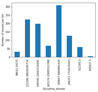
With decision tree discretization, each bin, that is, each prediction value in this case, does not necessarily contain the same number of observations. Let’s check that out with a visualization:
import matplotlib.pyplot as plt
train_t.groupby('GrLivArea')['GrLivArea'].count().plot.bar()
plt.ylabel('Number of houses')
plt.show()
Finally, we can determine if we have a monotonic relationship with the target after the transformation:
plt.scatter(test_t['GrLivArea'], y_test)
plt.xlabel('GrLivArea')
plt.ylabel('Sale Price')
plt.show()
Rounding the prediction value#
Sometimes, the output of the prediction can have multiple values after the comma, which makes the
visualization and interpretation a bit uncomfortable. Fortunately, we can round those values through
the precision
parameter:
disc = DecisionTreeDiscretiser(
bin_output="prediction",
precision=1,
cv=3,
scoring='neg_mean_squared_error',
variables=['LotArea', 'GrLivArea'],
regression=True)
disc.fit(X_train, y_train)
train_t= disc.transform(X_train)
test_t= disc.transform(X_test)
train_t.groupby('GrLivArea')['GrLivArea'].count().plot.bar()
plt.ylabel('Number of houses')
plt.show()
In this example, we are predicting house prices, which is a continuous target. The procedure for
classification models is identical, we just need to set the parameter regression
to False.
Discretization with interval limits#
In this section, instead of replacing the original variable values with the predictions of the decision tree, we will return the limits of the intervals. When returning interval boundaries, we need to set the precision to a positive integer.
disc = DecisionTreeDiscretiser(
bin_output="boundaries",
precision=3,
cv=3,
scoring='neg_mean_squared_error',
variables=['LotArea', 'GrLivArea'],
regression=True)
# fit the transformer
disc.fit(X_train, y_train)
In this case, when we explore the binner_dict_
attribute, we will see the interval limits instead
of the decision trees:
disc.binner_dict_
{'LotArea': [-inf, 8637.5, 10924.0, 13848.5, inf],
'GrLivArea': [-inf,
749.5,
808.0,
1049.0,
1144.5,
1199.0,
1413.0,
1438.5,
1483.0,
1651.5,
1825.0,
1969.5,
2386.0,
2408.0,
2661.0,
4576.0,
inf]}
The DecisionTreeDiscretiser()
will use these limits with pandas.cut
to discretize the
continuous variable values during transform:
train_t = disc.transform(X_train)
test_t = disc.transform(X_test)
print(train_t[['LotArea', 'GrLivArea']].head())
In the following output we see the interval limits into which the values of the continuous attributes were sorted:
LotArea GrLivArea
254 (-inf, 8637.5] (1199.0, 1413.0]
1066 (-inf, 8637.5] (1483.0, 1651.5]
638 (8637.5, 10924.0] (749.5, 808.0]
799 (-inf, 8637.5] (1651.5, 1825.0]
380 (-inf, 8637.5] (1651.5, 1825.0]
To train machine learning algorithms we would follow that up with any categorical data encoding method.
Discretization with ordinal numbers#
In the last part of this guide, we will replace the variable values with the number of bin into which the value was sorted. Here, 0 is the first bin, 1 the second, and so on.
disc = DecisionTreeDiscretiser(
bin_output="bin_number",
cv=3,
scoring='neg_mean_squared_error',
variables=['LotArea', 'GrLivArea'],
regression=True,
)
# fit the transformer
disc.fit(X_train, y_train)
The binner_dict_
will also contain the limits of the intervals:
disc.binner_dict_
{'LotArea': [-inf, 8637.5, 10924.0, 13848.5, inf],
'GrLivArea': [-inf,
749.5,
808.0,
1049.0,
1144.5,
1199.0,
1413.0,
1438.5,
1483.0,
1651.5,
1825.0,
1969.5,
2386.0,
2408.0,
2661.0,
4576.0,
inf]}
When we apply transform, DecisionTreeDiscretiser()
will use these limits with pandas.cut
to
discretize the continuous variable:
train_t = disc.transform(X_train)
test_t = disc.transform(X_test)
print(train_t[['LotArea', 'GrLivArea']].head())
In the following output we see the interval numbers into which the values of the continuous attributes were sorted:
LotArea GrLivArea
254 0 5
1066 0 8
638 1 1
799 0 9
380 0 9
Additional considerations#
Decision tree discretization uses scikit-learn’s DecisionTreeRegressor or DecisionTreeClassifier under the hood to find the optimal interval limits. These models do not support missing data. Hence, we need to replace missing values with numbers before proceeding with the disrcretization.
Tutorials, books and courses#
Check also for more details on how to use this transformer:
For tutorials about this and other discretization methods and feature engineering techniques check out our online course:
Or read our book:
Both our book and course are suitable for beginners and more advanced data scientists alike. By purchasing them you are supporting Sole, the main developer of Feature-engine.