BoxCoxTransformer

The Box-Cox transformation is a generalization of the power transformations family and is defined as follows:

y = (x**λ - 1) / λ,      for λ != 0
y = log(x),              for λ = 0

Here, y is the transformed data, x is the variable to transform and λ is the transformation parameter.

The Box Cox transformation is used to reduce or eliminate variable skewness and obtain features that better approximate a normal distribution.

The Box Cox transformation evaluates commonly used transformations. When λ = 1 then we have the original variable, when λ = 0, we have the logarithm transformation, when λ = - 1 we have the reciprocal transformation, and when λ = 0.5 we have the square root.

The Box-Cox transformation evaluates several values of λ using the maximum likelihood, and selects the optimal value of the λ parameter, which is the one that returns the best transformation. The best transformation occurs when the transformed data better approximates a normal distribution.

The Box Cox transformation is defined for strictly positive variables. If your variables are not strictly positive, you can add a constant or use the Yeo-Johnson transformation instead.

Uses of the Box Cox Transformation

Many statistical methods that we use for data analysis make assumptions about the data. For example, the linear regression model assumes that the values of the dependent variable are independent, that there is a linear relationship between the response variable and the independent variables, and that the residuals are normally distributed and centered at 0.

When these assumptions are not met, we can’t fully trust the results of our regression analyses. To make data meet the assumptions and improve the trust in the models, it is common practice in data science projects to transform the variables before the analysis.

In time series forecasting, we use the Box Cox transformation to make non-stationary time series stationary.

References

George Box and David Cox. “An Analysis of Transformations”. Read at a RESEARCH MEETING, 1964. https://rss.onlinelibrary.wiley.com/doi/abs/10.1111/j.2517-6161.1964.tb00553.x

BoxCoxTransformer

The BoxCoxTransformer() applies the BoxCox transformation to numerical variables. It uses SciPy.stats under the hood to apply the transformation.

The BoxCox transformation works only for strictly positive variables (>=0). If the variable contains 0 or negative values, the BoxCoxTransformer() will return an error. To apply this transformation to non-positive variables, you can add a constant value. Alternatively, you can apply the Yeo-Johnson transformation with the YeoJohnsonTransformer().

Python code examples

In this section, we will apply this data transformation to 2 variables of the Ames house prices dataset.

Let’s start by importing the modules, classes and functions and then loading the house prices dataset and separating it into train and test sets.

import matplotlib.pyplot as plt
from sklearn.datasets import fetch_openml
from sklearn.model_selection import train_test_split

from feature_engine.transformation import BoxCoxTransformer

data = fetch_openml(name='house_prices', as_frame=True)
data = data.frame

X = data.drop(['SalePrice', 'Id'], axis=1)
y = data['SalePrice']


X_train, X_test, y_train, y_test = train_test_split(
    X, y, test_size=0.2, random_state=42)

print(X_train.head())

In the following output we see the predictor variables of the house prices dataset:

      MSSubClass MSZoning  LotFrontage  LotArea Street Alley LotShape  \
254           20       RL         70.0     8400   Pave   NaN      Reg
1066          60       RL         59.0     7837   Pave   NaN      IR1
638           30       RL         67.0     8777   Pave   NaN      Reg
799           50       RL         60.0     7200   Pave   NaN      Reg
380           50       RL         50.0     5000   Pave  Pave      Reg

     LandContour Utilities LotConfig  ... ScreenPorch PoolArea PoolQC  Fence  \
254          Lvl    AllPub    Inside  ...           0        0    NaN    NaN
1066         Lvl    AllPub    Inside  ...           0        0    NaN    NaN
638          Lvl    AllPub    Inside  ...           0        0    NaN  MnPrv
799          Lvl    AllPub    Corner  ...           0        0    NaN  MnPrv
380          Lvl    AllPub    Inside  ...           0        0    NaN    NaN

     MiscFeature MiscVal  MoSold  YrSold  SaleType  SaleCondition
254          NaN       0       6    2010        WD         Normal
1066         NaN       0       5    2009        WD         Normal
638          NaN       0       5    2008        WD         Normal
799          NaN       0       6    2007        WD         Normal
380          NaN       0       5    2010        WD         Normal

[5 rows x 79 columns]

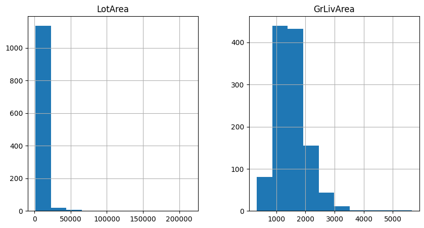
Let’s inspect the distribution of 2 variables in the original data with histograms.

X_train[['LotArea', 'GrLivArea']].hist(figsize=(10,5))
plt.show()

In the following plots we see that the variables are non-normally distributed:

Now we apply the BoxCox transformation to the 2 indicated variables. First, we set up the transformer and fit it to the train set, so that it finds the optimal lambda value.

boxcox = BoxCoxTransformer(variables = ['LotArea', 'GrLivArea'])
boxcox.fit(X_train)

With fit(), the BoxCoxTransformer() learns the optimal lambda for the transformation. We can inspect these values as follows:

boxcox.lambda_dict_

We see the optimal lambda values below:

{'LotArea': 0.0028222323212918547, 'GrLivArea': -0.006312580181375803}

Now, we can go ahead and transform the data:

train_t = boxcox.transform(X_train)
test_t = boxcox.transform(X_test)

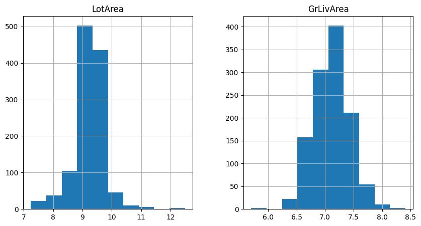
Let’s now examine the variable distribution after the transformation with histograms:

train_t[['LotArea', 'GrLivArea']].hist(figsize=(10,5))
plt.show()

In the following histograms we see that the variables approximate better the normal distribution.

If we want to recover the original data representation, we can also do so as follows:

train_unt = boxcox.inverse_transform(train_t)
test_unt = boxcox.inverse_transform(test_t)

train_unt[['LotArea', 'GrLivArea']].hist(figsize=(10,5))
plt.show()

In the following plots we see that the variables are non-normally distributed, because they contain the original values, prior to the data transformation:

Tutorials, books and courses

You can find more details about the Box Cox transformation technique with the BoxCoxTransformer() here:

• Jupyter notebook

For tutorials about this and other data transformation techniques and feature engineering methods check out our online courses:

Feature Engineering for Machine Learning

Feature Engineering for Time Series Forecasting

Or read our book:

Python Feature Engineering Cookbook

Our book and courses are suitable for beginners and more advanced data scientists alike. By purchasing them you are supporting Sole, the main developer of Feature-engine.